I started using Pigment 3 days ago and I´m trying to figure out how to recreate an Excel formula in the platform.

The excel formula I have is the following:
=INDEX($B$6:$M$6,MATCH($A9,$B$5:$M$5,0))*C$7


Basically my issue lies in he part of fixating the formula to one single cell.
 

the multiplication brings the correct result for the first cell in the Table I created, but the formula replicates to all cells in the row and I haven´t been able to figure out how to fixate the first part of the formula in order for the multiplication to only change cells for the last part of the formula (*C$7).

Can anyone share some guidance please?

Hi @Oscar Salazar , 

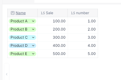
My assumption is that you for example you have products in B5:M5 and sales number of it in B6:M6. now you have a product in A9 and your formula above searches this product in B5:M5 and returns values from B6:M6 and then you want it to be multiplied by a number is C$7 and it should be changeable.

based on above, my suggestion for formula would be that, you create a transaction list but product as one of the dimension and Sales of it which covers above(B5:M5 & B6:M6) now create additional property and add the number (C7 for each product).
 

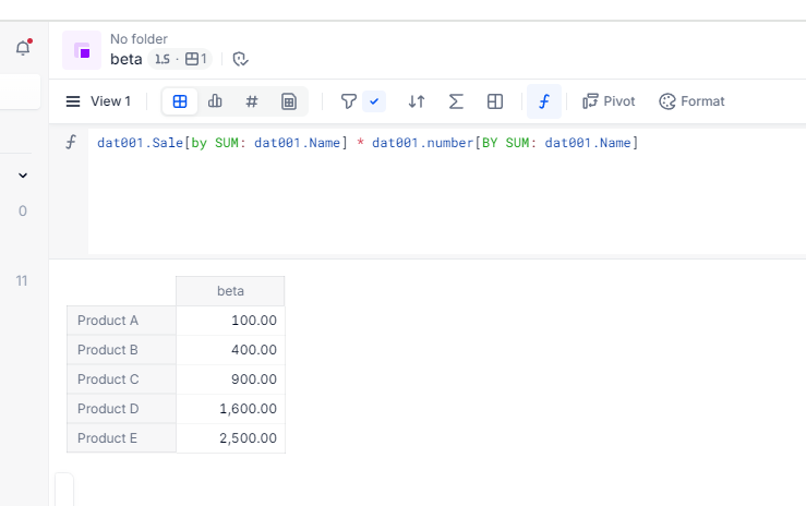
 Now create a metric as below and you should be able to see the excepted result.


Let me know if any questions


Index/Match & Vlookup is where Pigment is really different from Excel as we are a multi-dimensional tool.


the keyword is BY BY modifier | Community (pigment.com)

Look into the academy class:  Pigment and Multidimensionality

To go further, this article could be good: Multi Dimensional Modeling | Community (pigment.com)


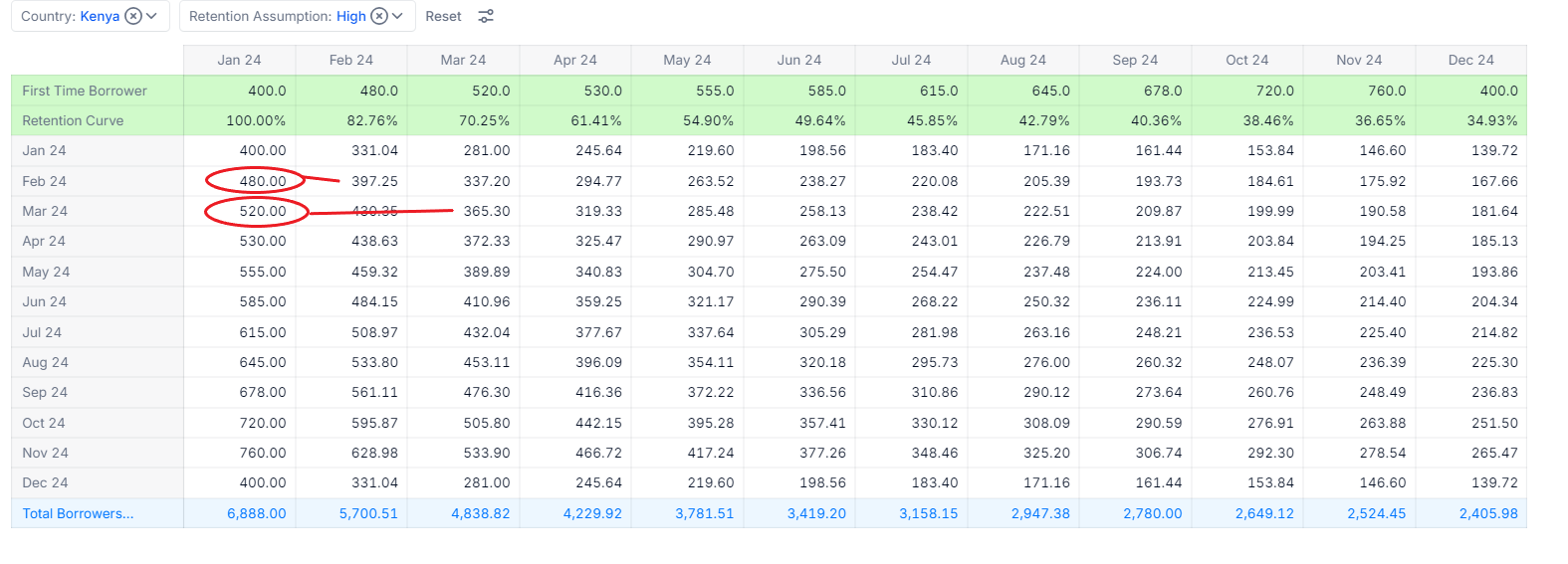
Hi @Nathan This as really helpfull, I figure out the formula that I needed but now I have another kind of issue.

The formula I used is: 'First Time Borrower'eby constant:Month."Jan 24"]*'Retention Curve' it works perfectly for Jan 24 row, but from Feb 24 I changed the “constant” to Feb 24 but I need the formula to start in column “Feb 24” and Jan 24 to be blank, for Mar 24 row the formula to start from column Mar 24 while Jan 24 and Feb 24 say blank. And repeat this for all months.

Any suggestions on how to make that change?


Reply