
Conditional formatting helps you visually explore and analyze data, detect critical issues, and identify patterns and trends. It makes it easier to highlight interesting cells or a range of cells, emphasize unusual values, and visualize data by using color scales.
A conditional format changes the appearance of cells (background color, font color, font style, borders, prefix and suffix) on the basis of conditions that you specify. If the conditions are true, the cell range is formatted; if the conditions are false, the cell range isn’t formatted. Conditional formatting is supported for Numbers, Text, Booleans, Dimensions and Dates. There are many built-in conditions that can be applied to create rules.
⚠️ Important
Conditional formatting is supported for Dimensions, Date, Number, Text, and Boolean data types.
Table of Contents
Apply a Rule
- Right click on the column or row you want to highlight.
- Select Conditional Formatting
- Select a condition from the menu.
For example, this could be Empty or Not Empty. Depending on the condition value, you can select the data type values you wish to apply it to. There are different conditions depending on your data type. - Confirm the Value type and Condition.
- Enter the value you wish to apply the formatting to.
- Select the different formatting options you wish to apply.
- If applicable, select the cells where you want to display this formatting.
- Click Done.
Want to take your conditional formatting a step further? In Pigment you can also apply conditional formatting based on another Metric. This allows you to apply conditional formatting on a Metric or Dimension Item based on the outcome of a Metric within the same table. Check out Apply Conditional Formatting Based on Another Metric for more information.
Conditional Formatting Rules
| Option | Definition |
| Empty | Format cells that are empty |
| Not empty | Format cells that are not empty |
| Lower than | Format cells that are lower than a <number> |
| Lower than or equal to | Format cells that are lower than or equal to a <number> |
| Greater than | Format cells that are greater than a <number> |
| Greater than or equal to | Format cells that are greater than or equal to a <number> |
| Equal to | Format cells that are equal to a <number> |
| Not equal to | Format cells that are not equal to a <number> |
| Between | Format cells that are between a <number1> and <number2> |
| Not between | Format cells that are not between a <number1> and <number2> |
| Color scale | Format either the cell text or the cell background by using a gradation of two colors with <number1> as min and <number2> as max. You can choose to add a midpoint <number3> to use a three color gradation. The shade of the color represents higher or lower values. |
Formatting options
There are different formatting options that you can apply to cells that meet the conditions set in the rule.
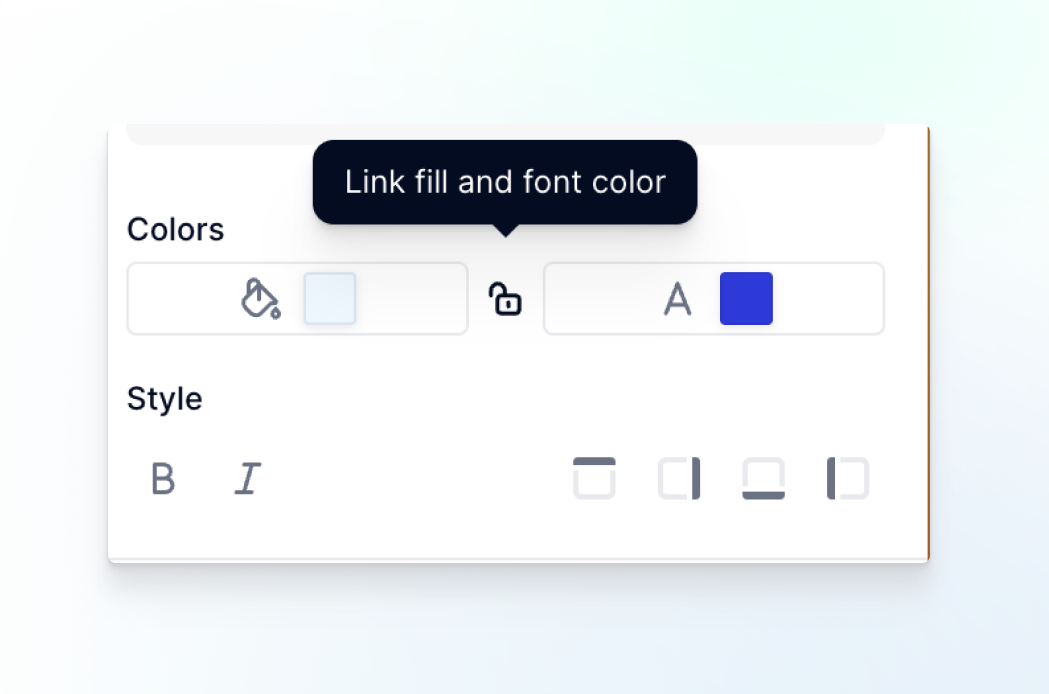
- Background and Text color. You can link two colors by clicking the Lock icon. If the lock icon is on, the text and the background are used together in future selections. Click the Lock icon to unlink the associated colors if you prefer a different customization.
- Font. Select B for bold and I for italic formatting.
- Cell borders. Applies a border to selected cell walls. The selection is applied to each individual cell that is highlighted.
Manage or Edit the order on which Conditional formatting rules apply
The order in which conditional formatting rules are evaluated also reflects their relative importance: the higher a rule is on the list of conditional formatting rules, the more important it is.
This means that where two conditional formatting rules conflict with each other, the rule that’s higher on the list is applied and the rule that is lower on the list isn’t applied.
To reorder the rules, open the Format panel, click Conditional, and reorder the formatting rules using the up and down arrows beside each rule.
Edit Conditional Formatting Rules
Open the Format Panel and under the Conditional tab, select the rule you want to edit.
Clear Conditional Formatting Rules
Open the Format Panel and under the Conditional tab, click on the Delete icon that appears next to the rule you want to remove.
Cell Status Conditional Formatting Rules
You can use conditional formatting in specific Views to highlight cells that can be input and cells that have been overridden. This is a powerful way to maintain clarity and consistency when using grids that require input from multiple users.
There are two types of cell status indicator that can be activated through the conditional formatting panel:
- Input cells. A gray border is added to the cell if it can be edited.
- Overridden cells. A blue vertical bar is displayed indicating data that is the result of a formula that has been manually overridden.
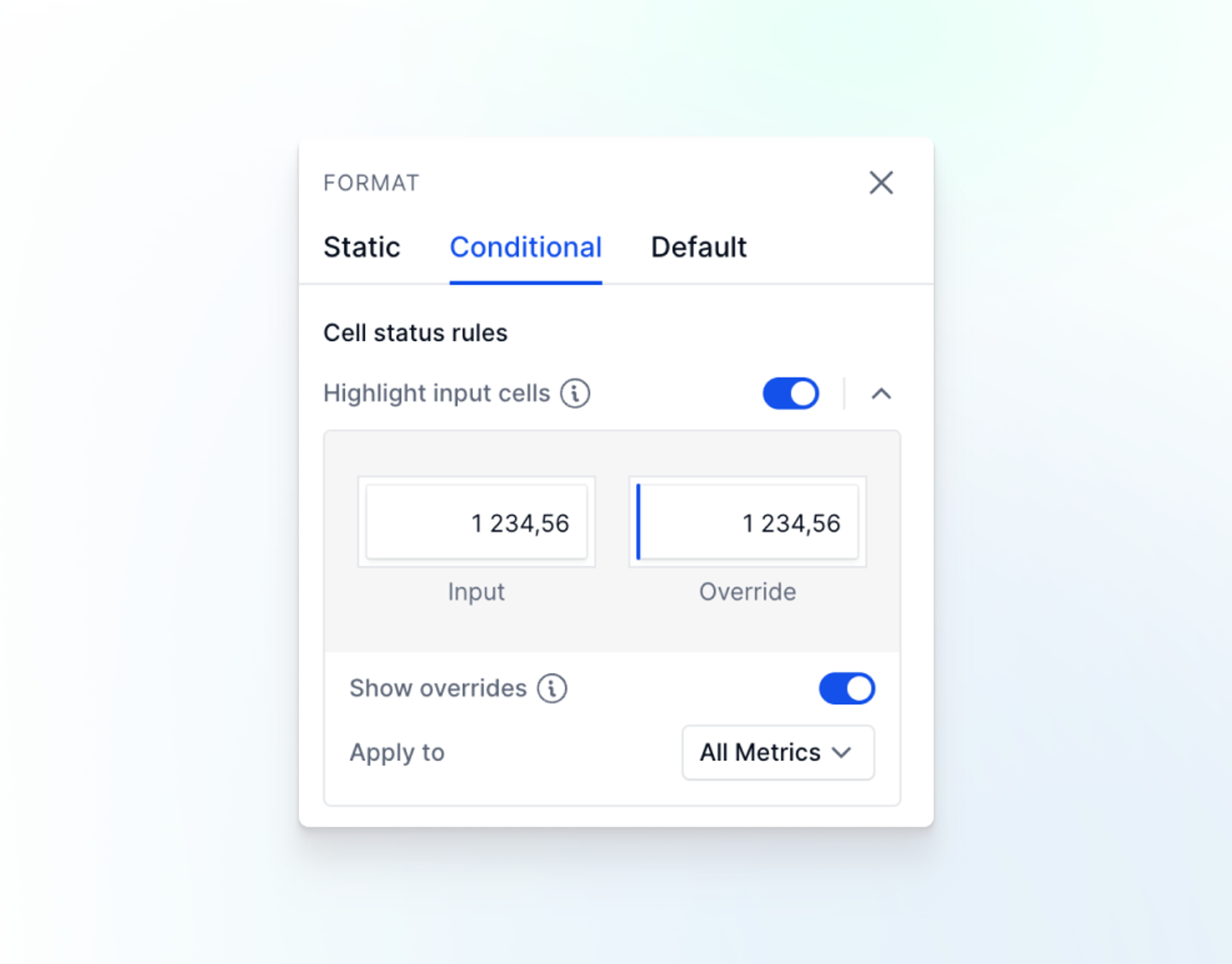
To highlight cells that can be input or cells that have been overridden:
- Expand the View.
- Click Format.
- Select the Conditional formatting tab.
- Toggle on Highlight input cells.
- Select the following options if applicable:
- Show Overrides: A blue vertical bar will appear around the cells that have been overridden.
- Select Metrics: By default, the formatting will apply to all metrics. Use the Apply to dropdown to choose specific Metrics to format. For example, if a Table has ten Metrics, but only five are relevant for user input, you can select those five Metrics.