Pigment formula syntax and basic operations share some similarities with Excel. The difference is that in Pigment, your data is stored in ‘Blocks’. This article sets out some of the key similarities and differences between the two platforms.
Referencing data: Pigment versus Excel
-
Pigment holds data in Blocks, which include Transaction Lists, Dimension Lists and Metrics. You directly reference their names in formulas
(Revenue * Growth), instead of cells like in Excel(B2 * D42). -
Unlike Excel, the formulas you enter in Pigment apply directly to all the cells of a Block. To perform operations between those Blocks, Pigment just needs to know their names.
-
Since Pigment is multi-dimensional, you'll need to learn a few tricks to aggregate and allocate data. Check out the Aggregating data in formulas article.
Benefits of Pigment’s Approach
Organizing data into Dimensions and Metrics allows for a more flexible, scalable, and intuitive way to manage complex datasets and write formulas.
Instead of relying on individual cell references like in Excel, which can become error-prone and difficult to trace, Pigment’s Blocks are inherently linked and multi-dimensional. This allows users to slice and aggregate data efficiently across multiple Dimensions (e.g. time, product, or region) and apply consistent logic at scale.
It also enhances data transparency and collaboration, as every piece of data is clearly defined and easier to audit. You never have to ‘drag’ the formula down like in Excel, because it automatically applies to all cells in a Metric, which is particularly useful when you add new products or employees in your Dimension Lists.
TIP
You can recreate certain Excel functions by switching your Metric’s View to Sheet View.
Example 1: basic formulas
In Excel you might apply basic formulas as below. You derive your Revenue forecast for 2025 by arranging columns of input data, including actual Revenue for 2024 and a Growth estimate, side by side. Next, you copy and paste an output formula down column D, as below:

In Pigment, the data in each column would be held in different Blocks. Blocks used as an axis to break out your data are called Dimensions. You create a Dimension called Country as in the image:

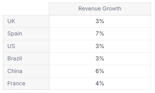
Revenue for 2024 and your growth forecasts are numerical input data. These Blocks are Metrics broken out by the Country Dimension, as in the image:
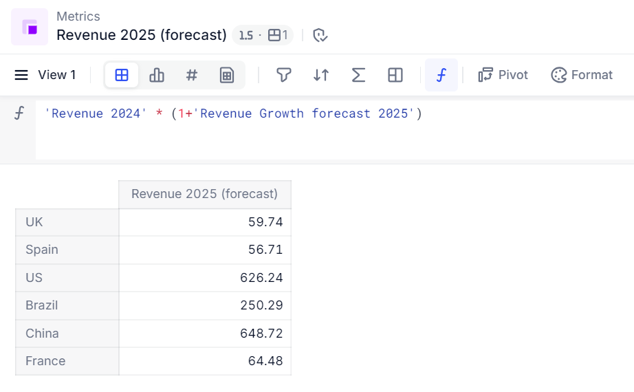
To obtain your desired output, you create a Metric Revenue 2025 (forecast), and add one formula which applies to all cells. It references the Blocks’ names instead of a cell range:'Revenue 2024' * (1+'Revenue Growth forecast 2025')
Example 2: VLOOKUP versus Pigment formulas
In Excel’s VLOOKUP() you search for the value of one cell in a range and retrieve data from an offset cell, as below:

In Pigment, your data would be in Blocks, such as:
- A Dimension called Product defining the names of your products. You add a column giving Price as a Property of each product. Learn more about Properties here.
- A Metric of Monthly sales (units), broken out by the new Product Dimension.

Next, to obtain Revenue by product by month as in the Excel above, you multiply the Monthly sales (units) Metric by the products’ prices. As prices are a Property of Product, you reference them using the following syntax (see Write your First Formula for more information on syntax for Properties):
'Monthly sales units' * Product.Price

Pigment can handle additional complexity. Imagine that the above case is just one of several countries you sell in. Your prices are different in each country. Price is no longer a single fixed attribute associated with each product. Now you need price data according to country and product line, requiring creation of a new Dimension Country.
So you create a Metric of Price by country as follows:

Your Revenue formula now references your new Price Metric instead of a static Price Property:
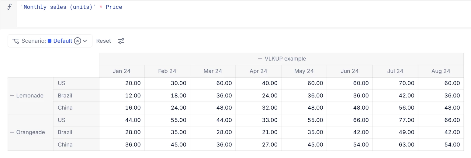
'Monthly sales (units)' * Price
This single formula calculates for all data points. Using Pivot allows both the Product and the Country Dimensions to be shown in the rows, as below:
Example 3: VLOOKUP versus BY FIRSTNONBLANK
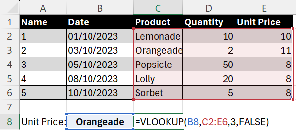
Similar to Example 2 above, VLOOKUP() could look up a product name and return a Unit Price as follows, in the below case “Orangeade” at a price of 11:
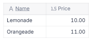
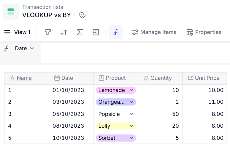
In Pigment, the input data looks as follows, held in a Transaction list type Block:
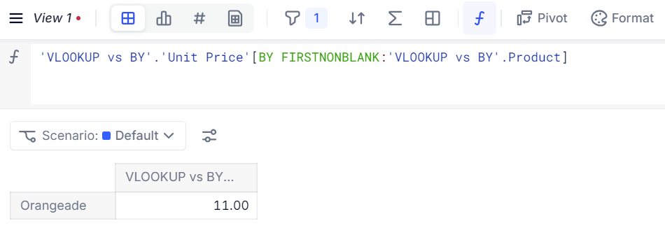
To retrieve price information, we create a Metric, whose formula references the above Transaction list’s Unit Price Property, then breaks it out by product using BY and FIRSTNONBLANK to call the first data point per product, ignoring any preceding blanks. A filter is applied to isolate data for Orangeade only, as in the image below:
For more information, see the BY Modifier article.
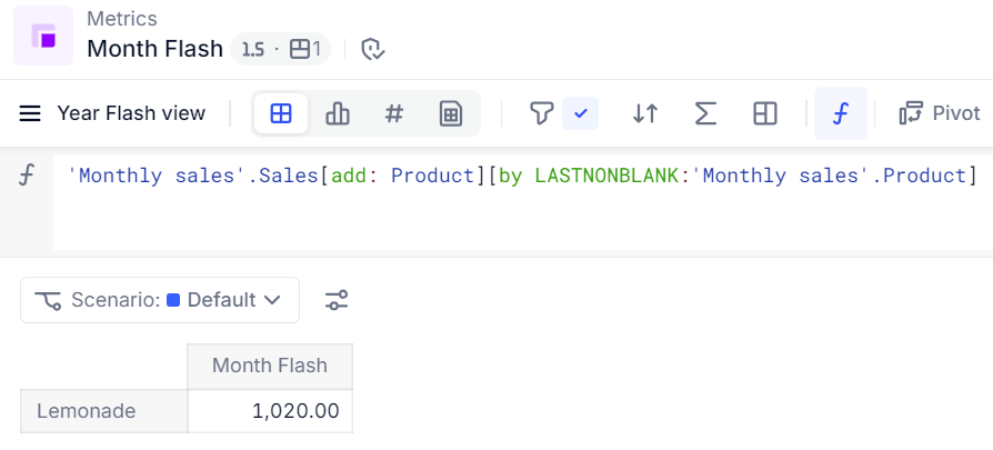
Example 4: XLOOKUP versus BY LASTNONBLANK
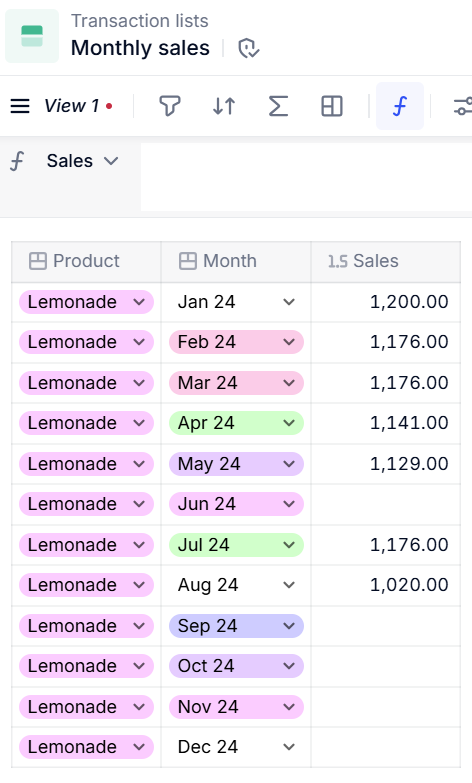
Often you need to retrieve the latest data point in a series—for example, raw sales data accumulates for current month in an accounting spreadsheet. In Excel, you would use XLOOKUP(), starting at the end of the series and finding the first non blank value. Below, XLOOKUP() finds “1020”:

In Pigment your raw data is imported into a Block of type Transaction list as follows:
To retrieve your current month sales figure you create a Metric with a BY LASTNONBLANK modifier. For more information, see the BY Modifier article.
Example 5: SUMIFS
In Excel your raw Revenue data may be in a list, and you use SUMIFS() as follows to obtain totals for various products by country:

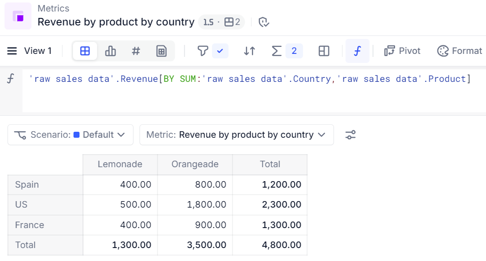
In Pigment, your raw data is input or imported to a Transaction list called raw sales data. You call it into a Metric Revenue by product by country, with a totals column and row added using the Sum aggregator as follows:
